SysML Parametric Diagrams: Modeling Constraints & Performance

Systems engineering relies heavily on precise mathematical relationships to validate design decisions before physical prototypes are built. SysML parametric diagrams serve as the backbone for this analytical work. They allow engineers to define equations, constraints, and performance metrics within the broader context of a system model. By integrating structural and behavioral aspects with mathematical logic, these diagrams enable rigorous verification of system capabilities.

This guide explores the mechanics of modeling constraints and performance. It covers the foundational elements, the construction of constraint blocks, the flow of data through binding connectors, and strategies for maintaining model integrity. The focus remains on the technical application of the standard to ensure systems meet their defined requirements.

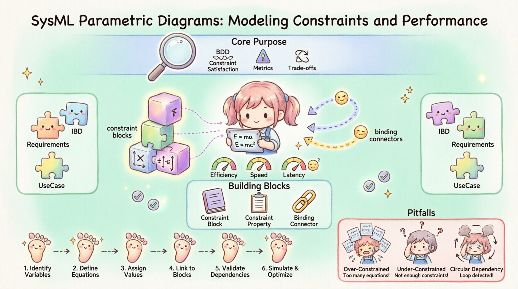
Chibi-style infographic summarizing SysML parametric diagrams for modeling constraints and performance, featuring cute engineer character, constraint blocks with equations like F=ma, binding connectors, performance metrics gauges, 6-step implementation workflow, common pitfalls warnings, and integration with BDD/IBD/Requirements diagrams in soft pastel kawaii aesthetic

🔍 Understanding the Core Purpose

Parametric diagrams differ from standard structural diagrams by introducing algebraic relationships. While a Block Definition Diagram defines the parts of a system, a parametric diagram defines how those parts interact mathematically. This is essential for performance analysis.

Constraint Satisfaction: Verifying if a design meets physical limits like temperature, pressure, or power.
Performance Metrics: Calculating outcomes such as fuel efficiency, response time, or throughput.
Trade-off Analysis: Evaluating how changes in one variable affect others across the system.

Without these diagrams, a system model remains a static description. With them, it becomes a dynamic simulation environment capable of answering “what if” questions regarding system performance.

🧱 Foundational Building Blocks

To construct a valid parametric model, one must understand the specific elements available within the language. These elements work together to define the boundaries of the system.

1. Constraint Blocks

A constraint block is a specialized type of block used to define a specific relationship. Unlike a regular block representing a physical component, a constraint block represents a rule or an equation. It acts as a container for the mathematical logic.

Properties: Variables within the constraint block (e.g., mass, force, velocity).
Constraints: The actual equations linking the properties (e.g., force = mass * acceleration).
Reusability: Constraint blocks can be reused across different system models to ensure consistency in calculations.

2. Constraint Properties

While constraint blocks define the rule, constraint properties are the instances of that rule. A single constraint block can be instantiated multiple times to model different scenarios or components.

Binding: A constraint property binds to specific blocks in the system architecture.
Aggregation: Multiple constraint properties can be aggregated to form complex performance models.

3. Binding Connectors

Binding connectors are the lines that link properties of constraint blocks to properties of structural blocks. They define the flow of values between the system structure and the mathematical model.

Data Flow: They pass values from one variable to another.
Consistency: They ensure that a variable in the structural block matches the variable in the constraint block.
Direction: Unlike flow connectors in activity diagrams, binding connectors are typically undirected in terms of data dependency, focusing on equality.

📊 Structuring Constraint Models

Organizing constraints effectively is critical for maintainability. A chaotic model leads to confusion during validation. The following table outlines the relationship between structural elements and parametric elements.

Structural Element	Parametric Equivalent	Purpose
Block	Constraint Block	Defines physical component vs. Defines mathematical rule
Property	Constraint Property	Represents a specific instance of a component vs. Represents a specific instance of a rule
Flow Connector	Binding Connector	Connects signals/materials vs. Connects variables for calculation
Requirement	Constraint Equation	Defines a goal vs. Defines the mathematical boundary

🧮 Modeling Equations and Logic

The heart of a parametric diagram is the equation. These equations can range from simple arithmetic to complex differential equations depending on the complexity of the system.

Algebraic Constraints

These are the most common form, used for steady-state analysis. They relate variables at a single point in time.

Linear Equations: Used for basic calculations like cost or mass summation.
Non-Linear Equations: Required for aerodynamic drag or thermodynamic efficiency.

Conditional Constraints

Sometimes, equations only apply under certain conditions. SysML allows for the definition of conditional logic within constraints.

If-Then Logic: A constraint applies only if a specific boolean property is true.
Thresholds: Performance is valid only if variables stay within defined ranges.

Discrete vs. Continuous

Understanding the nature of the variables is vital for simulation.

Continuous Variables: Represent quantities that can take any value (e.g., temperature, voltage).
Discrete Variables: Represent distinct states (e.g., on/off, gear selection).

🚀 Performance Analysis Strategies

Once the model is built, the goal is to derive performance metrics. This process transforms raw data into actionable engineering insights.

1. Defining Performance Metrics

Metrics are the outputs of the system. They should be clearly defined as properties within the constraint blocks.

Efficiency: Ratio of output energy to input energy.
Reliability: Probability of failure over a specific time period.
Latency: Time taken for a signal to propagate through the system.

2. Simulation and Verification

Simulation involves solving the equations to find values for unknown variables. Verification ensures the calculated values meet the requirements.

Input Parameters: Fixed values provided to the model (e.g., ambient temperature).
Output Parameters: Calculated values (e.g., maximum operating speed).
Constraint Solving: The process of finding a solution that satisfies all equations simultaneously.

3. Sensitivity Analysis

This technique tests how changes in input variables affect the output. It helps identify critical components.

High Sensitivity: Small changes in input cause large changes in output.
Low Sensitivity: Input changes have minimal impact on output.

This analysis directs resources toward the most critical design areas.

🛠️ Implementation Workflow

Building a parametric model follows a logical sequence. Skipping steps often leads to inconsistencies later in the engineering lifecycle.

Identify Variables: List all physical quantities that influence performance.
Create Constraint Blocks: Define the mathematical rules governing these quantities.
Instantiate Properties: Place the constraint blocks onto the diagram.
Bind Connectors: Link the constraint properties to the structural block properties.
Define Values: Assign known values to input properties.
Validate: Run the solver to check for contradictions or unsolvable equations.

⚠️ Common Pitfalls and Troubleshooting

Even experienced engineers encounter issues with parametric models. Recognizing these patterns helps in maintaining a robust system.

1. Over-Constrained Systems

This occurs when there are more equations than unknown variables. The system may become impossible to solve.

Symptom: Solver reports contradictory constraints.
Fix: Review redundant equations and remove unnecessary constraints.

2. Under-Constrained Systems

This happens when there are more unknown variables than equations.

Symptom: The solver cannot determine a unique value for a variable.
Fix: Add more constraints or assign default values to variables.

3. Circular Dependencies

Variables depend on each other in a loop without a clear starting point.

Symptom: Solver fails to converge.
Fix: Break the loop by introducing a time step or a known reference value.

4. Naming Inconsistencies

Using different names for the same physical quantity across different blocks.

Symptom: Binding connectors do not link correctly.
Fix: Enforce a standard naming convention for all variables.

🔗 Integration with Other Diagrams

Parametric diagrams do not exist in isolation. They integrate deeply with other SysML diagram types to provide a complete system view.

Block Definition Diagram (BDD)

The BDD defines the hierarchy. The parametric diagram references the blocks defined here. Changes in the BDD (like adding a new block) must be reflected in the parametric model.

Internal Block Diagram (IBD)

The IBD defines the interfaces between blocks. Binding connectors in the parametric diagram often link to ports defined in the IBD. This ensures that the mathematical model aligns with the physical interface.

Requirement Diagram

Requirements define the goals. Parametric constraints often map directly to requirements. For example, a requirement for “Maximum Temperature” becomes a constraint equation checking that limit.

Use Case Diagram

Use cases define the operational scenarios. Different scenarios may require different sets of constraint blocks to be active or modified.

📈 Best Practices for Maintenance

To keep the model useful over time, adherence to best practices is essential. This ensures the model remains accurate as the system evolves.

Modularization: Group related constraints into separate constraint blocks. This reduces complexity.
Documentation: Add notes to constraint blocks explaining the origin of the equation (e.g., empirical data, theoretical derivation).
Version Control: Track changes to equations. A change in a formula can impact the entire system performance.
Abstraction: Hide complex calculations behind high-level properties. This keeps the diagram readable.
Validation: Regularly run the solver to ensure no new contradictions have been introduced.

🌐 Advanced Topics in Performance Modeling

For complex systems, standard algebraic constraints may not suffice. Advanced modeling techniques are available for specific scenarios.

Time-Dependent Constraints

Systems that change over time require differential equations. This allows for the modeling of dynamic behavior.

Differentiation: Modeling rates of change (e.g., acceleration).
Integration: Modeling accumulated values (e.g., total fuel consumed).

Probabilistic Modeling

When inputs are uncertain, deterministic equations are insufficient. Probabilistic constraints allow for the modeling of risk.

Distributions: Using statistical distributions for input variables.
Monte Carlo: Running multiple simulations to determine probability of failure.

Multi-Domain Modeling

Systems often involve electrical, mechanical, and thermal domains. Parametric diagrams can link variables across these domains.

Power Conversion: Relating electrical power to mechanical torque.
Heat Transfer: Relating electrical resistance to thermal dissipation.

🏁 Summary of Key Concepts

Effective use of SysML parametric diagrams requires a solid understanding of both system structure and mathematical logic. By following the guidelines below, engineers can create models that provide genuine value.

Start with Requirements: Ensure every constraint traces back to a system requirement.
Keep it Modular: Break complex systems into manageable constraint blocks.
Validate Often: Check for over-constrained and under-constrained states regularly.
Document Logic: Explain the “why” behind every equation.
Integrate Early: Link parametric models to structural diagrams from the beginning.

The integration of performance modeling into the system architecture ensures that decisions are data-driven. It reduces the risk of design errors and provides a clear path from concept to validation. By treating constraints as first-class citizens in the model, the engineering process becomes more rigorous and reliable.

🔍 Detailed Checklist for Model Review

Before finalizing a parametric diagram, use this checklist to ensure quality.

Check Item	Pass Criteria
Variable Naming	All variables have unique, descriptive names.
Equation Consistency	Units are consistent across all equations.
Connectivity	All binding connectors link to valid properties.
Requirement Traceability	Every constraint links to a requirement ID.
Solver Status	The model solves without errors or warnings.
Documentation	Equations have comments explaining their source.

Adhering to this checklist minimizes errors and ensures the model remains a reliable asset throughout the system lifecycle. The goal is not just to create a diagram, but to create a tool for engineering decision-making.