


Relational databases are built on the foundation of tables and rows, a structure designed for flat data. However, the real world rarely adheres to such simplicity. Organizations, file systems, comment threads, and category trees all exist in hierarchical structures. Representing these parent-child relationships in a standard Entity Relationship Diagram (ERD) requires specific design patterns that maintain data integrity while allowing for efficient retrieval.
When you attempt to map a tree structure onto a flat schema, you encounter the classic tension between normalization and performance. This guide explores the core techniques for modeling hierarchical data, evaluating the trade-offs of each approach to help you design robust systems.
🧩 The Challenge of Flat Schemas
An Entity Relationship Diagram typically visualizes entities as boxes and relationships as lines. In a standard relationship, one table links to another via a Foreign Key. This works perfectly for a many-to-many or one-to-many scenario where the direction is fixed. But what happens when a category can have sub-categories, which can have sub-sub-categories, potentially infinitely?
Standard relational models struggle with variable depth. A flat table cannot easily store a path of arbitrary length. To solve this, we must adapt the schema to store the hierarchy explicitly. There are three primary patterns used by data architects to achieve this:
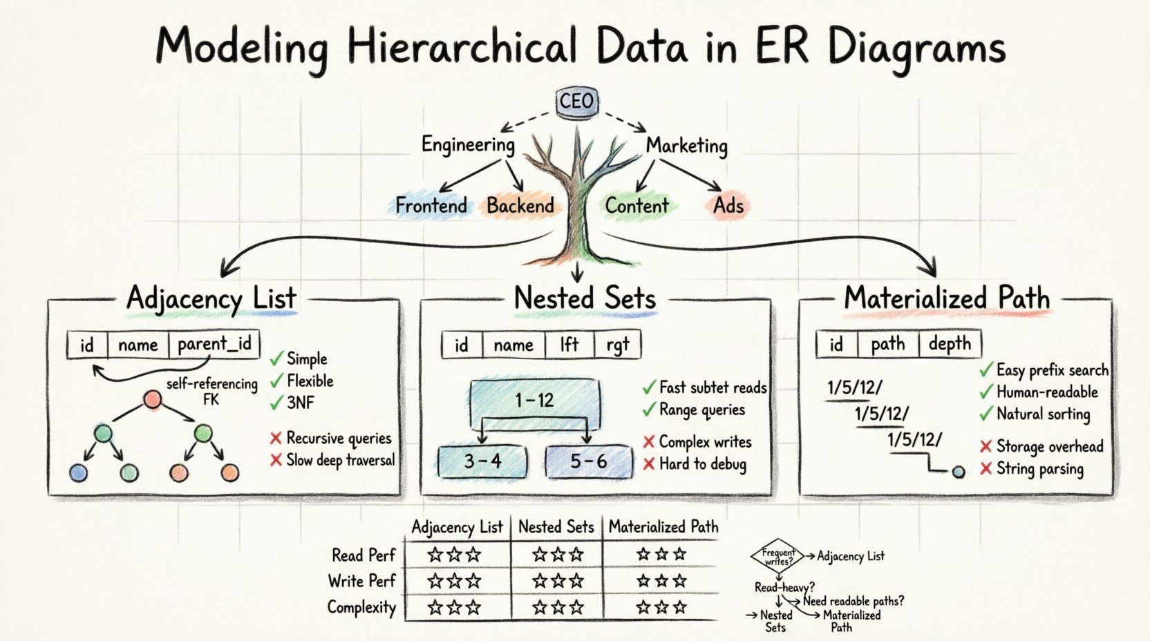
- Adjacency List: Storing the parent ID within the child record.
- Nested Sets: Assigning left and right values to define ranges.
- Path Enumeration: Storing the full path from the root to the current node.
🔗 The Adjacency List Model
The Adjacency List is the most common and straightforward method for representing hierarchy in a standard ERD. It relies on a self-referencing relationship. This means a single table contains a column that references its own primary key.
📐 Schema Structure
In this model, you create a single table to hold the data. Each row represents a node in the tree. The critical addition is a column, often named parent_id or ancestor_id, which holds the unique identifier of the parent node. If a node is at the top of the hierarchy, this column contains a null value.
Consider a table for Department:
- id: The unique primary key for the department.
- name: The display name of the department.
- parent_id: The ID of the superior department (nullable for top-level).
✅ Advantages
- Simplicity: The schema is intuitive and easy to understand for developers and database administrators.
- Flexibility: Moving a subtree is simple; you only need to update the
parent_idof the root node of that subtree. - Normalization: It adheres well to Third Normal Form (3NF) as data is not repeated.
❌ Disadvantages
- Query Complexity: Retrieving all descendants requires recursive queries or application-side processing.
- Performance: Deep traversals can be slow without specific indexing strategies or recursive common table expressions (CTEs).
- Referential Integrity: While foreign keys help, circular references can still occur if constraints are not strictly enforced.
🌲 The Nested Set Model
The Nested Set model transforms the tree structure into a set of intervals. Instead of tracking parent pointers, each node is assigned two numbers: left and right. These values represent the node’s position in a pre-order traversal of the tree.
📐 Schema Structure
Imagine a tree where the root node is the entire set. As you traverse the tree, you increment a counter. When you enter a node, you record the current count as left. When you finish processing that node and all its children, you record the count as right. The right value is always greater than the left value.
A Category table would look like this:
- id: Unique identifier.
- name: Category name.
- lft: The left boundary value.
- rgt: The right boundary value.
✅ Advantages
- Fast Retrieval: Fetching a subtree is a simple range query using
BETWEENlogic. - Efficiency: Read performance is superior for large, deep trees compared to adjacency lists.
❌ Disadvantages
- Write Cost: Inserting or moving a node is expensive. You must update the
lftandrgtvalues of many other nodes to maintain the integrity of the intervals. - Complexity: The logic is difficult to implement and debug without dedicated library support.
🛣️ Path Enumeration and Materialized Paths
Path Enumeration methods store the lineage of a node as a string or a delimited list. This approach is often called the Materialized Path pattern. It combines the simplicity of the adjacency list with the readability of the path.
📐 Schema Structure
In this model, each record stores the full path from the root. For example, in a file system model, a file might have a path string like /home/user/documents/report.txt. In a database, this is often stored as a delimited string within the column, such as 1/5/12/.
The table includes:
- id: Primary key.
- path: A string representing the lineage.
- depth: An integer indicating how many levels deep the node is.
✅ Advantages
- Easy Traversal: You can find all descendants by matching the path prefix.
- Readability: The data is human-readable and easy to debug.
- Sorting: Sorting by the path string often yields the correct tree order naturally.
❌ Disadvantages
- Storage Overhead: Long paths can consume significant storage space.
- String Parsing: Queries often require string manipulation functions, which can be slower than integer comparisons.
📊 Comparative Analysis
Choosing the right model depends heavily on your read-to-write ratio and the depth of your hierarchy. The following table outlines the characteristics of each method.
| Feature | Adjacency List | Nested Sets | Materialized Path |
|---|---|---|---|
| Read Performance | Low to Medium | High | Medium to High |
| Write Performance | High | Low | Medium |
| Implementation Complexity | Low | High | Medium |
| Supports Deep Trees | Yes | Yes | Yes (with limits) |
| Query Logic | Recursive | Range Scan | Prefix Match |
⚙️ Performance Considerations
When modeling hierarchy, you must consider how the database engine handles the data. Indexing strategies play a critical role regardless of the model chosen.
- Adjacency List: Index the
parent_idcolumn heavily. This allows the database to quickly locate all children of a specific node without scanning the entire table. - Nested Sets: Index both
lftandrgt. Composite indexes can optimize range queries significantly. - Materialized Path: Index the
pathcolumn. Depending on the database, a prefix index might be beneficial for filtering sub-trees.
🛠️ Maintenance and Updates
Data models are not static. As your organization grows, your hierarchy will change. Moving a node from one branch to another is a common operation that impacts each model differently.
🔄 Moving Nodes
In an Adjacency List, moving a node is a single update statement. You change the parent_id of the root of the subtree. However, you must ensure no circular references are created.
In a Nested Set model, moving a node is complex. It involves recalculating the lft and rgt values for all nodes in the destination subtree to make room for the moved node. This is often a transactional operation involving multiple table updates.
In a Materialized Path model, you update the path string of the moved node and all its descendants. This requires updating the path for every child, which can be a heavy write operation for large trees.
🎯 Best Practices for Data Modeling
To ensure your ERD remains maintainable and performant, follow these guidelines when implementing hierarchical structures.
- Use Clear Naming Conventions: Avoid generic names like
col1. Useparent_id,ancestor_id,lft, orrgtexplicitly. - Enforce Constraints: Use database constraints to prevent circular references. A node cannot be its own ancestor.
- Limit Depth: While technically possible, extremely deep hierarchies (e.g., more than 10 levels) often indicate a design flaw. Consider flattening the structure if possible.
- Document the Choice: Since these patterns are not standard SQL features, document which pattern is used in the schema documentation.
- Consider Hybrid Approaches: Some systems combine Adjacency Lists with Materialized Paths to balance read and write performance.
🧠 Choosing the Right Strategy
There is no single “correct” answer for every scenario. The decision rests on the specific requirements of your application.
- Choose Adjacency List if: Your data changes frequently, and the hierarchy depth is moderate. This is the safest default for most general-purpose applications.
- Choose Nested Sets if: You have a read-heavy application where data is rarely moved, and you need to retrieve large subtrees quickly.
- Choose Materialized Path if: You need human-readable paths (like URLs) and the hierarchy depth is relatively shallow.
Understanding these structural nuances allows you to design databases that scale. By selecting the appropriate pattern for your Entity Relationship Diagram, you ensure that your data remains consistent, accessible, and efficient throughout the lifecycle of the system.